Week 7 - Nov. 2

Location Our Normal Classroom

Theme Networks: social, knowledge, and others. Agent Based Models.

Have Read for Today

Brughmans, Tom. 2010. “Connecting the dots: Towards archaeological network analysis” Oxford Journal of Archaeology, 29:3, 277–303, https://doi.org/10.1111/j.1468-0092.2010.00349.x. Available through our library proxy
Mills, Barbara. 2017. “Social Network Analysis in Archaeology”. Annual Review of Anthropology 46:379-397. https://www.annualreviews.org/docserver/fulltext/anthro/46/1/annurev-anthro-102116-041423.pdf?expires=1752075004&id=id&accname=guest&checksum=9CB9F30B21C6A2BA1F9243F7947ECB4D
Romanowska, I., Crabtree, S. A., Harris, K. and Davies, B. 2019: Agent-Based Modeling for Archaeologists: Part 1 of 3. Advances in Archaeological Practice 7 (2). 178–84. link (This also comes with a tutorial for the Netlogo language; feel free to read that too if you want)
Optional: Graham S, Yates D, El-Roby A, Brousseau C, Ellens J, McDermott C. Relationship Prediction in a Knowledge Graph Embedding Model of the Illicit Antiquities Trade. Advances in Archaeological Practice. 2023;11(2):126-138. doi:10.1017/aap.2023.1. The point of sharing this piece with you is to illustrate that there are ways of exploring the latent spaces between the nodes and edges of a network, and that this is a way of surfacing ideas ‘hiding’ in our knowledge that we didn’t initially spot.

The Plan A discussion of how a networked perspective on archaeological data opens up new ways of seeing the past. Then, a further excursion into how archaeological networks can be reanimated.

Skill Building

We’ll build a network of a small farming community from a small rural cemetery
We’ll load a networked representation of the Roman Empire into a Google Colab notebook and calculate some network perspectives on it.
We’ll try to build an agent based model of information (or disease?) diffusion on top of the Roman empire’s urban topology

Homework By Friday at noon, have your research compendium for this week complete and in github. You might want to consider the perils of looking at the world through a network lens - and the potentials. Have you encountered this kind of approach in your history classes? What would your other professors make of all this?

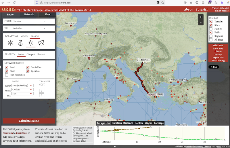
The ORBIS geospatial network model of the Roman world: https://orbis.stanford.edu/.

ORBIS is a multimodal, seasonally variable transportation network model available at orbis.stanford.edu. The model provides for practically unlimited permutations by allowing users to limit modes, change movement cost, and adjust time of year. However, it is as a more simple network that ORBIS can be usefully integrated into other research, such as historical environmental reconstruction or agent-based modeling set in the Roman world. (Scheidel, Weiland and Arcenas 2014)

Historical Cemetery Network Dataset

I’ll give you some information I cooked up regarding a small family cemetery. Your goal is to create a new python or R notebook in Google Colab where you load the data in and do some analyzes.

take this data, and make a new text file (remember, you never use Word for something like this. Use a text editor (and if you don’t recall what I mean by that, just ask). Represent the data provided to you below as an ‘edgelist’ where you list out the relationships. You need to have at least a ‘source’ and ‘target’ column, eg:
```
source,target
alice,bob
```
You might want to have more columns. When you save the txt file, CHANGE THE FILE EXTENSION to end with .csv, eg: graveyard_net.csv.

Then,

make a new python or R notebook
load the data in
visualize the data
determine one or two metrics for the data.

Hint In python, you can load the data with pandas: edges_df = pd.read_csv('edges.csv')

In R, you can load it in with igraph: links <- read.csv("edges.csv", header=T, as.is=T)

Each family seemed to have its own section in the cemetery.

Thompson Family

| Person | Birth Year | Death Year | Notes | |——–|————|————|——-| | John Thompson | 1820 | 1889 | Patriarch, miller | | Mary Thompson | 1823 | 1891 | Wife of John | | Sarah Thompson | 1847 | 1923 | Eldest daughter | | Robert Thompson | 1849 | 1901 | Son, took over mill | | James Thompson | 1851 | 1934 | Youngest son | | Alice Thompson | 1872 | 1945 | Robert’s wife |

Hayes Family

| Person | Birth Year | Death Year | Notes | |——–|————|————|——-| | William Hayes | 1825 | 1895 | Blacksmith, business partner to John | | Elizabeth Hayes | 1828 | 1901 | Wife of William | | Thomas Hayes | 1850 | 1918 | Son, continued blacksmithing | | Margaret Hayes | 1852 | 1925 | Daughter, schoolteacher | | Robert Thomson and Margaret Hayes | | joint headstone? | | Catherine Miller | 1875 | 1942 | Daughter, Thomas | | David Hayes | 1877 | 1950 | Thomas’s son |

Miller Family

| Person | Birth Year | Death Year | Notes | |——–|————|————|——-| | Samuel Miller | 1815 | 1882 | Town doctor | | Ruth Miller | 1818 | 1885 | Wife of Samuel | | Benjamin Miller | 1845 | 1920 | Son, also doctor | | Hannah Miller | 1848 | 1929 | Daughter, midwife | | Edward Miller | 1870 | 1935 | Benjamin’s son | | Catherine Hayes | 1875 | 1942 | Edward’s wife |

Clark Family

| Person | Birth Year | Death Year | Notes | |——–|————|————|——-| | Charles Clark | 1830 | 1905 | Store owner | | Emma Clark | 1833 | 1908 | Wife of Charles | | Frank Clark | 1855 | 1940 | Son, inherited store | | Lucy Clark | 1857 | 1932 | Daughter | | Henry Clark | 1880 | 1955 | Frank’s son | | Rose Clark | 1882 | 1960 | Frank’s wife | | Hannah … | ? | ? | Frank’s first wife? |

Wilson Family

| Person | Birth Year | Death Year | Notes | |——–|————|————|——-| | George Wilson | 1822 | 1890 | Farmer | | Martha Wilson | 1825 | 1893 | Wife of George | | Joseph Wilson | 1848 | 1915 | Son, farmer | | Mary Wilson | 1850 | 1928 | Daughter | | Peter Wilson | 1875 | 1940 | Joseph’s son | | Anna Wilson | 1878 | 1945 | Joseph’s wife | | Charles Clark and Mary Wilson | | | Joint headstone? |

Some code to get you started

If you choose to try this exercise using Python, see if you can work out how to repurpose the code notebook we used to explore ORBIS on your data.

If you want to try R:

In colab, change the runtime to use R. Drag and drop your data into the file tray. Then use the code below to get you started. Do not just dump this all into a single block. Try to maintain one block = one main operation. And then use text blocks between the code blocks to keep track of your thoughts etc.

# install igraph; this might take a long time
# you only run this line the first time you install igraph:
install.packages('igraph')
# a lot of stuff gets downloaded and installed.
# 
# now tell RStudio you want to use the igraph pacakge and its functions:
library('igraph')

# now let's load up the data by putting the csv files into nodes and links.
# we're keeping the first row as a 'header'

nodes <- read.csv("nodes.csv", header=T, as.is=T)
links <- read.csv("edges.csv", header=T, as.is=T)
#examine data
head(nodes)
head(links)

#we are going to tell igraph that the network is directed, that the relationship Alice to Bob is different than Bob's to Alice. This isn't always a critical distinction to make and depends on your dataset.
#AND - we're going to do this just from the edge data
#Create network from edges only - igraph will infer the nodes
net <- graph_from_data_frame(d=links, directed=T)

#(if we wanted to include the node data specifically, we could do this:
# net <- graph_from_data_frame(d=links, vertices=nodes, directed=T)
# see the difference?
# Calculate closeness centrality
closeness_cent <- closeness(net, normalized = TRUE)

# Histogram
hist(closeness_cent, 
     breaks = 20,
     main = "Distribution of Closeness Centrality",
     xlab = "Closeness Centrality",
     ylab = "Frequency",
     col = "lightgreen",
     border = "white")
abline(v = mean(closeness_cent), col = "red", lwd = 2, lty = 2)

# Network plot colored by closeness
close_colors <- colorRampPalette(c("lightblue", "darkgreen"))(100)
V(net)$color <- close_colors[as.numeric(cut(closeness_cent, breaks = 100))]

plot(net, 
     layout = layout_with_fr,
     vertex.size = closeness_cent * 50 + 5,  # Scale by closeness
     vertex.color = V(net)$color,
     vertex.frame.color = "white",
     edge.color = "gray50",
     edge.arrow.size = 0.5,
     vertex.label = NA,
     main = "Network: Closeness Centrality")

# Calculate betweenness centrality
betweenness_cent <- betweenness(net, normalized = TRUE)

# Histogram
hist(betweenness_cent, 
     breaks = 20,
     main = "Distribution of Betweenness Centrality",
     xlab = "Betweenness Centrality",
     ylab = "Frequency",
     col = "orange",
     border = "white")
abline(v = mean(betweenness_cent), col = "red", lwd = 2, lty = 2)

# Network plot colored by betweenness
between_colors <- colorRampPalette(c("lightblue", "darkorange"))(100)
V(net)$color <- between_colors[as.numeric(cut(betweenness_cent, breaks = 100))]

plot(net, 
     layout = layout_with_fr,
     vertex.size = sqrt(betweenness_cent) * 10 + 5,  # Square root scaling
     vertex.color = V(net)$color,
     vertex.frame.color = "white",
     edge.color = "gray50",
     edge.arrow.size = 0.5,
     vertex.label = NA,
     main = "Network: Betweenness Centrality")
# Detect communities using modularity
communities <- cluster_louvain(as.undirected(net))  # Convert to undirected for community detection
modularity_score <- modularity(communities)

# Print modularity score
cat("Modularity score:", modularity_score, "\n")
cat("Number of communities:", length(communities), "\n")

# Histogram of community sizes
community_sizes <- sizes(communities)
hist(community_sizes, 
     breaks = 10,
     main = paste("Distribution of Community Sizes\nModularity =", round(modularity_score, 3)),
     xlab = "Community Size",
     ylab = "Frequency",
     col = "purple",
     border = "white")

# Network plot colored by community
community_colors <- rainbow(length(communities))
V(net)$color <- community_colors[membership(communities)]

plot(net, 
     layout = layout_with_fr,
     vertex.size = 8,
     vertex.color = V(net)$color,
     vertex.frame.color = "white",
     edge.color = "gray50",
     edge.arrow.size = 0.5,
     vertex.label = NA,
     main = paste("Network: Communities (Modularity =", round(modularity_score, 3), ")"))